Google Meet Link: https://meet.google.com/nsa-kdpq-ysa
Github Repository Link: https://github.com/galava-shubhang/MPC-Rover

Aim

To compare Pure Pursuit Control (PPC) with Model Predictive Control (MPC) for rover path tracking in a 2D simulated environment, focusing on accuracy, obstacle avoidance, computational cost, and scalability.

Introduction

On this pale-blue dot we call Earth, what else can cars do if they can already navigate our streets autonomously? Could similar tech explore distant planets or map uncharted terrains in space? Imagine rovers autonomously exploring distant planets, mapping uncharted terrains, or navigating environments we’ve never dared to step in — all without constant human input. [1]

It takes at least 5 minutes for a signal from Earth to reach Mars, making piloting rovers nearly impossible. Many rovers have been damaged by the unforgiving Martian terrain (like so). Thankfully though, we can see into the future with the power of MPC (Model Predictive Control).

The vastness of space is full of unknowns, and efficient navigation is critical for making those unknowns a little more reachable. That’s where our project would come in handy: Simulating Rover Paths with MPC. MPC is widely used in scenarios where precision and efficiency are critical, such as autonomous driving, robotics, and industrial automation. In our project, we would use MPC to control a rover's movement along a path. It would ensure the vehicle follows the desired trajectory while maintaining the best speed and steering control, even taking the attempt one notch higher - introducing dynamic obstacles in the path to be followed by the rover.

Pure Pursuit Control (PPC) coupled with the Bicycle Model (BM) is another approach for navigation of a rover (more on them in the next section!) - so we also analysed and compared the performance of the PPC+BM model and the MPC model against a few decisive parameters like path tracking accuracy, computational cost, obstacle avoidance, energy efficiency and scalability in a 2D space with dynamic path planning given some predefined obstacles and constraints.

Technologies Used

MATLAB

Path Planning Algorithms

MPC Model

PPC Model

Bicycle Model

Literature Survey

1. Motion planning, also known as path planning, is a computational problem that aims to find a sequence of valid configurations that moves the object from the source to the destination. A basic path planning problem is to compute a continuous path that connects a start configuration S and a goal configuration G, while avoiding collision with known obstacles. The robot and obstacle geometry is described in a 2D or 3D workspace, while the motion is represented as a path in (possibly higher-dimensional) configuration space.

2. Model Predictive Control (MPC) is an advanced control strategy that guides a system (like a vehicle) by predicting its future behaviour based on a mathematical model. Unlike simple feedback controllers, MPC looks ahead, forecasts potential outcomes, and chooses the best action to minimise errors or meet particular objectives.  [1]

3. Pure Pursuit Control (PPC) is an approach that allows the rover to follow a predetermined path by calculating a target point on the path ahead of the rover and adjusting the steering angle to minimise the distance between its current heading and this point. Pure pursuit is a tracking algorithm that calculates the curvature that will move a vehicle from its current position to some goal position. The whole point of the algorithm is to choose a goal position some distance ahead of the vehicle on the path. The name pure pursuit comes from the analogy we use to describe the method. We tend to think of the vehicle as chasing a point on the path some distance ahead - it is pursuing that moving point. That analogy is often used to compare this method to how humans drive. We tend to look far in front of the car and head toward that spot. This lookahead distance changes as we drive to reflect the twist of the road and vision occlusions. [2, 3] 

4. Control Systems are the "brains" of a robot, enabling it to perceive its surroundings, process information, and execute tasks accurately and efficiently. These systems range from simple open-loop to sophisticated ML-driven solutions, ensuring robots can operate efficiently and adaptively. They involve various components and strategies to command and regulate a robot's behaviour, including movement, actions, and interactions with its environment.

5. MATLAB is a programming and numeric computing platform that millions of engineers and scientists use to analyse data, develop algorithms, and create models.

6. The Bicycle Model (BM) is a simplified way of representing a vehicle, like a rover, by reducing its four wheels to just two — one at the front and one at the back. This makes it easier to model how the rover changes direction as it moves [1, 2]. Let’s break down the key components of the model:

• Position (x, y): The rover’s location at any given moment.
• Yaw (θ): This is the rover’s orientation, or the angle it makes relative to its starting direction.
• Velocity (v): The rover’s speed in a straight line.
• Steering Angle (δ): This controls how sharply the rover turns.

Where:

• L is the wheelbase of the rover.
• a is the acceleration input, determined by the control system.

Methodology 

Implementation of the PPC and MPC Models

The MATLAB script (linked here) simulates a 2D rover following a path using two control techniques: Pure Pursuit Control (PPC) and Model Predictive Control (MPC). The simulation begins by setting time parameters (time step for each iteration T, number of simulation steps steps), rover properties (distance between front and rear axles L, constant linear velocity v), and the predefined path as a smooth sinusoidal curve. Static circular obstacles are also introduced. The PPC section starts with the function pure_pursuit_simulation, where the rover iteratively finds a lookahead point on the path and computes the steering angle (delta) using geometric relationships. The rover's pose is updated each step, and its motion is visualised using scatter. 

The MPC part begins with mpc_simulation, initialising the state vector [x, y, theta, velocity] and defining prediction horizon [N], control limits, and cost matrices Q and R. The controller solves an optimisation problem in each iteration using fmincon to find optimal control inputs over the prediction horizon. The cost function (mpc_cost) penalises deviation from the path, control effort, obstacle proximity, high speeds, and sharp steering changes. Obstacles are modelled as circles, and the rover avoids them through penalisation instead of hard constraints.

The rover_dynamics function updates the state based on bicycle model kinematics. The Bicycle Model is a simplified way to represent a vehicle's motion using just two wheels: one in front and one in the rear, like a bicycle. It captures the essential dynamics of turning and moving, making it ideal for path tracking algorithms like Pure Pursuit and Model Predictive Control. It captures turning behaviour using the steering angle (delta) and velocity (v). Both simulations visually plot rover movement to compare PPC’s simplicity against MPC’s predictive precision. This explains the working of the code. The demo of the simulation is under the Results section below.

The MPC Model with Dynamic Obstacles

The MATLAB code simulates the path of a rover in a 2D environment using MPC and dynamic obstacles. The aim is to guide the rover to the predicted target without collisions. The code can be found here or in the GitHub repository mentioned below.

The key features of this model include:

1. MPC controller - At each simulation step, it predicts future rover states over a prediction horizon N and optimises control inputs like acceleration and velocity accordingly.
2. Dynamic obstacles - Obstacles which move with pre-defined velocities. They change their position at each step of the simulation.
3. Rover dynamics - The rover's motion is modelled using a simple bicycle model, considering its speed, acceleration and position.
4. Visualisation - The simulation shows the rover's path, obstacles and the predicted target.
5. Flexibility - Additional features like boundary wrapping and collision prediction can be added in the code as required.

The code flow is as follows:

1. Initialisation: Sets up simulation parameters, obstacle locations, rover initial state, and plotting.
2. Main loop: The main loop updates dynamic obstacles, runs MPC to get optimal controls, moves the rover, and checks if the target is reached.
3. MPC Controller: Uses fmincon to find the best set of control inputs that guide the rover toward the target while avoiding obstacles.
4. Cost Function: Penalises distance to the target, control input effort, being too close to obstacles, and exceeding max speed.  

The simulation ends when the rover reaches the target or the time runs out. The demo of the simulation is under the Results section below.

Results

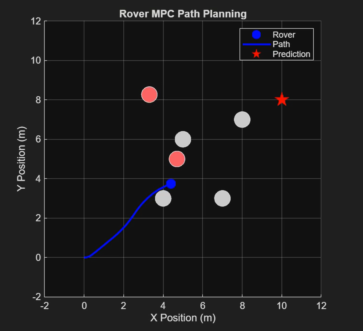
MPC Model Simulation

Video of the Demo can be found here. This is a demo of the MPC Model in action; it simulates the path of a rover in a 2D environment. The blue dot represents the rover, the pink dot represents the dynamic obstacles, the white dots are static obstacles, and the red star is the target/intended destination of the rover. The MPC model guides the rover to the predicted target without any collisions, in real time, as shown by the blue curve representing the path.

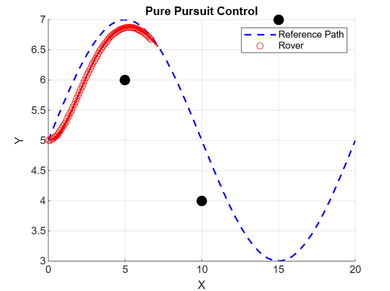
PPC Model Simulation

Video of the Demo can be found here. This is a demo of the PPC+BM model in action; it simulates the path of a rover in a 2D environment. The red circle represents the rover (at each time), and the black dots are static obstacles. The Pure Pursuit model guides the rover along the pre-defined path (the blue curve representing the path) without any collisions, in real time.

Comparison between PPC and MPC Models

1. Computational Cost: PPC is lightweight, making it easy for low-power onboard systems. MPC requires solving constrained optimisation problems repeatedly, needing more processing power.
2. Obstacle Avoidance: PPC does not inherently avoid obstacles; thus, one must add separate sensors or logic. MPC can plan trajectories considering obstacles directly, making it safer in cluttered environments.
3. Energy Efficiency: MPC’s optimisation leads to smoother control inputs, reducing energy waste from abrupt manoeuvres. PPC may cause jerky steering.
4. Scalability: PPC works well for simple, smooth paths but struggles when the environment or goals become more complex. MPC scales better in handling multiple constraints, but at a higher computation cost.

Conclusions

The 2D simulation compared Pure Pursuit Control (PPC) and Model Predictive Control (MPC) on a dynamically planned path with obstacles. MPC showed higher path tracking accuracy and smoother trajectories, especially in tight turns, but at a higher computational cost. PPC was faster and simpler, performing well on smoother paths. MPC handled obstacle avoidance more robustly, while PPC scaled better for larger systems.

Future Scope

1. Implement a hybrid PPC-MPC system based on path conditions.
2. Extend to multi-rover coordination with collision avoidance.
3. Add terrain modelling for rough surfaces or Mars-like environments.
4. Integrate real-time path replanning and learning-based control.
5. Expand to 3D simulation and potential hardware validation.

References

1. Blog on MPC - Our primary reference.
2. Blog on PPC.
3. Implementation of the Pure Pursuit Path Tracking Algorithm.
4. Model Predictive Control  Applications For Planetary Rovers.
5. Iterative learning-based model predictive control for mobile robots in space applications.
6. Static Obstacle Avoidance for Rover Vehicles Using Model Predictive Controller.

Project Github Repository

All the simulation files and source codes can be found here in the GitHub Repository or here in Google Drive.

Acknowledgement

As executive members of IEEE NITK, we are incredibly grateful for the opportunity to learn and work on this project under the prestigious name of the IEEE NITK Student Chapter. We want to extend our heartfelt thanks to IEEE for providing us with the funds to complete this project successfully.

The Team

Mentors: 

• Akanksh Vishwan Patil [231MT006]
• Shubhang S. Galagali [231MT049]

Mentees:

• Sanjit Kumar Srinivasan [241ME348]
• Vikram Prem Kumar [241EC163]
• Reuben Abraham Jacob [241EE147]
• Nandini Eswaran  [241CH026]
• Chavada Vishva Anilkumar [241EC212]