

Modelling and Evaluation of PEMFC Performance
Abstract
Abstract
I. INTRODUCTION
Proton Exchange Membrane Fuel Cells (PEMFCs) hold potential as a green technology for future energy owing to their high efficiency, minimal emissions, and wide applicability in combined heat and power (CHP) schemes. Drawing from recent work (Zhang et al., 2024), our project targets the simulation and optimization of a Ballard PEMFC system through the use of MATLAB/Simulink.
II. LITERATURE REVIEW
A. Introduction
Proton Exchange Membrane Fuel Cells (PEMFCs) are widely researched for their high efficiency, low operating tem- perature, and suitability for automotive and stationary applica- tions. They utilize hydrogen and oxygen to generate electrical energy through an electrochemical reaction, producing water and heat as by-products. The performance of PEMFCs is determined by several key factors, including electrochemical kinetics, mass transport, and thermal management.
B. Theoretical Background
The working principle of PEMFCs is based on the electro- chemical reaction occurring at the anode and cathode. Hydro- gen molecules dissociate at the anode, releasing protons and electrons. The protons migrate through the proton exchange membrane, while electrons travel through an external circuit, generating electricity. At the cathode, oxygen molecules com- bine with electrons and protons to form water.
The main electrochemical reactions are:
Anode: \(\mathrm{H}_2 \rightarrow 2\mathrm{H}^+ + 2e^- \) (1)
Cathode: \(\frac{1}{2} \mathrm{O}_2 + 2\mathrm{H}^+ + 2e^- \rightarrow \mathrm{H}_2\mathrm{O} \) (2)
C. Equations
The output voltage of a PEMFC can be determined by:
\(V_{\text{cell}} = E - V_{\text{act}} - V_{\text{ohm}} - V_{\text{con}} \) (3)
E is the thermodynamic potential (V), Vact is the activation, overpotential (V), Vohm is the ohmic overpotential (V), Vcon is the concentration overpotential (V).
The following formula can be used to calculate the thermodynamic potential:
\({E = 1.229 - 0.85 * 10^{-3} * (T_P - T_{ref}) + \frac{RT}{2F} ln P_{H2} + \frac{RT}{4F} ln P_{O2}} \) (4)
where TPEMFC is the cell temperature (K), Tref is the reference temperature (K), PH2 is the hydrogen partial pressure (kPa), PO2 is the oxygen partial pressure (kPa).
The empirical formula derived from the experimental data is used to express the activation overpotential, where ξ1, ξ2, ξ3, and ξ4, are empirical parameters, CO2 is the oxygen concentration, I is the cell output current (A):
\(V_{\text{act}} = \xi_1 + \xi_2 T_P + \xi_3 T_P \ln P_{{O2}} + \xi_4 T_P \ln I \) (5)
The ohmic overpotential can be determined by the Ohm’s law, Rm is the membrane resistance:
\(V_{\text{ohm}} = I R_m \) (6)
The concentration overpotential can be expressed by the following formula, where m and n are empirical parameters:
\(V_{\text{con}} = m \exp\left(\frac{nI}{A}\right) \) (7)
The fuel cell stack output power can be expressed as, where N is the number of fuel cells:
\(P_{\text{elc}} = N V_{\text{cell}} I \) (8)
The heat dissipated from the inside of the stack includes the gas heat dissipation, radiant heat dissipation, and cooling water heat dissipation:
\(Q_{\text{dis}} = Q_{\text{gas}} + Q_{\text{atm}} + Q_{\text{cl}} \) (9)
where Qgas is the gas heat dissipation power (kW), Qatm is radiated heat dissipation power (kW), Qcl is the cooling water heat dissipation power (kW).
The amount of heat contained in the gas entering the stack can be expressed as:
\(Q_{\text{gas,in}} = \left( {N}_{\text{in,an,H}_2} C_{\text{H}_2} + {N}_{\text{in,an,H}_2\text{O}} C_{\text{H}_2\text{O}} \right) (T_{\text{in,an}} - T_0) + \left( {N}_{\text{in,ca,air}} C_{\text{air}} + {N}_{\text{in,ca,H}_2\text{O}} C_{\text{H}_2\text{O}} \right) (T_{\text{in,ca}} - T_0) \) (10)
where Nin,an,H2 is the hydrogen flow rate at the anode inlet (mol/s), Nin,an,H2O is the anode inlet water vapor flow rate (mol/s), Nin,ca,air is the cathode inlet air flow rate (mol/s), Nin,ca,H2O is the cathode inlet water vapor flow rate (mol/s), CH2 is the specific heat capacity of hydrogen (kJ/(kg K)), Cair is the specific heat capacity of air (kJ/(kg K)), Cg,H2O is the specific heat capacity of water vapor (kJ/(kg K)), T0 is the standard ambient temperature (K).
\({ Q_{out} = (N_{out,ca,O2} C_{O2} + N_{out,ca,N2} C_{N2})(T_{out,ca} - T_0) + (N_{out,ca,H2O} C_{H2O} + N_{out,ca,H2O,l} C_{H2O})(T_{out,ca} - T_0) + (N_{out,an,H2} C_{H2} + N_{out,an,H2O} C_{H2O})(T_{out,an} - T_0) } \) (11)
Nout,ca,O2 is the oxygen flow rate at the cathode outlet (mol/s), Nout,ca,N2 is the nitrogen flow rate at the cathode outlet (mol/s), Nout,ca,H2O is the water vapor flow rate at the cathode outlet (mol/s), Nout,ca,H2O, l is the flow rate of liquid water at the cathode outlet (mol/s), Nout,an,H2 is the hydrogen flow rate at the anode outlet (mol/s), Nout,an,H2O is the anode outlet water vapor flow rate (mol/s), CN2 is the specific heat capacity of nitrogen (kJ/(kg K)), Cl,H2O is the specific heat capacity of liquid water (kJ/(kg K)).
These were for the voltage and power part of model. For the efficiency part:
\({n_{H2} = S_{H2} * N_{rec,an,H2}} \) (12)
\(\eta_{\text{elec}} = \frac{P_{\text{elc}}}{\dot{n}_{{H2}} *\Delta H_{{H2}}} \) (13)
\({ \eta_{th} = (W_{ex,cl} * C_{l,H2O} * \Delta T) / (\dot n_{H2} * \Delta H_{H2}) } \) (14)
where SH2 is the stoichiometric ratio of H2, n.H2 is the molar flow rate of H2 ,ηelec is the electrical efficiency of the system, ηth is the thermal efficiency of the system. Overall Efficiency is the addition of both electrical and thermal efficiency.
III. METHODOLOGY
We modelled all these equations into Simulink- MATLAB. Simulink supports closed-loop design and control logic, which is crucial for optimizing PEMFC performance under varying conditions. We can create custom blocks to represent specific components of PEMFC systems, such as membrane electrode assemblies, gas flow networks, and cooling systems.
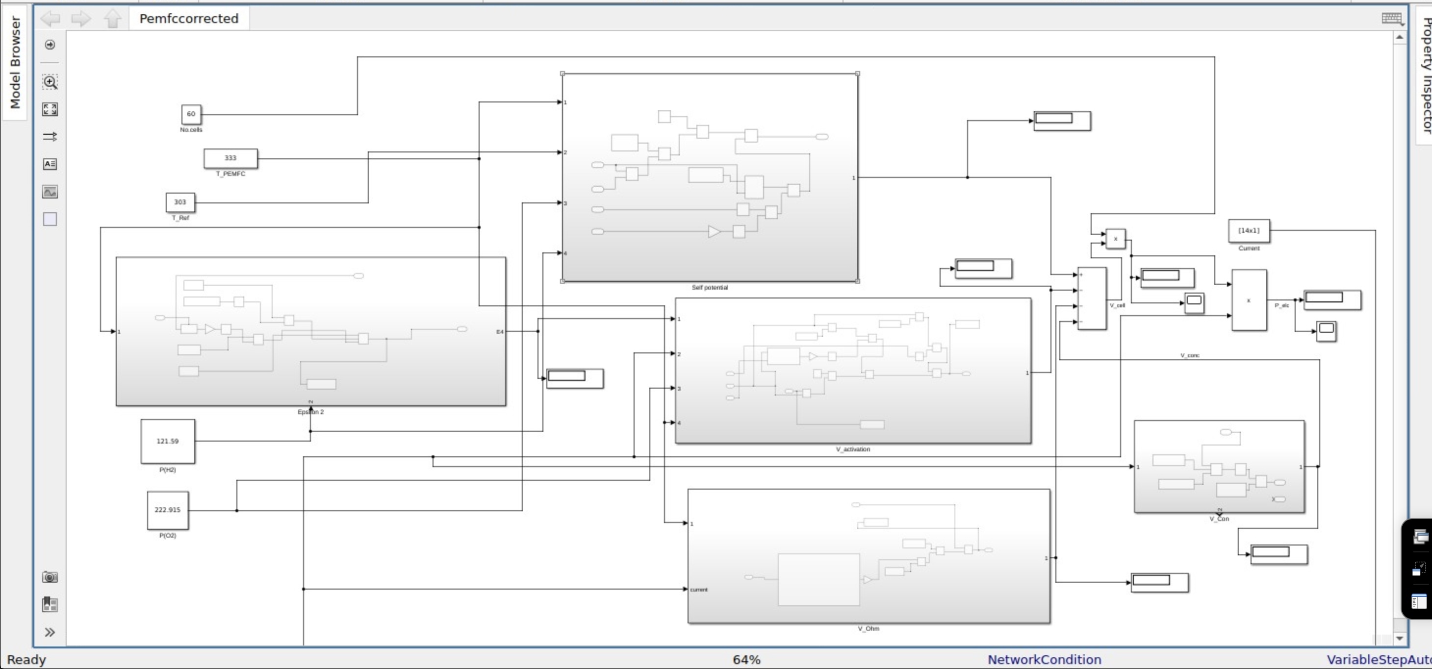
Fig. 1. Simulink model for Voltage and Power.
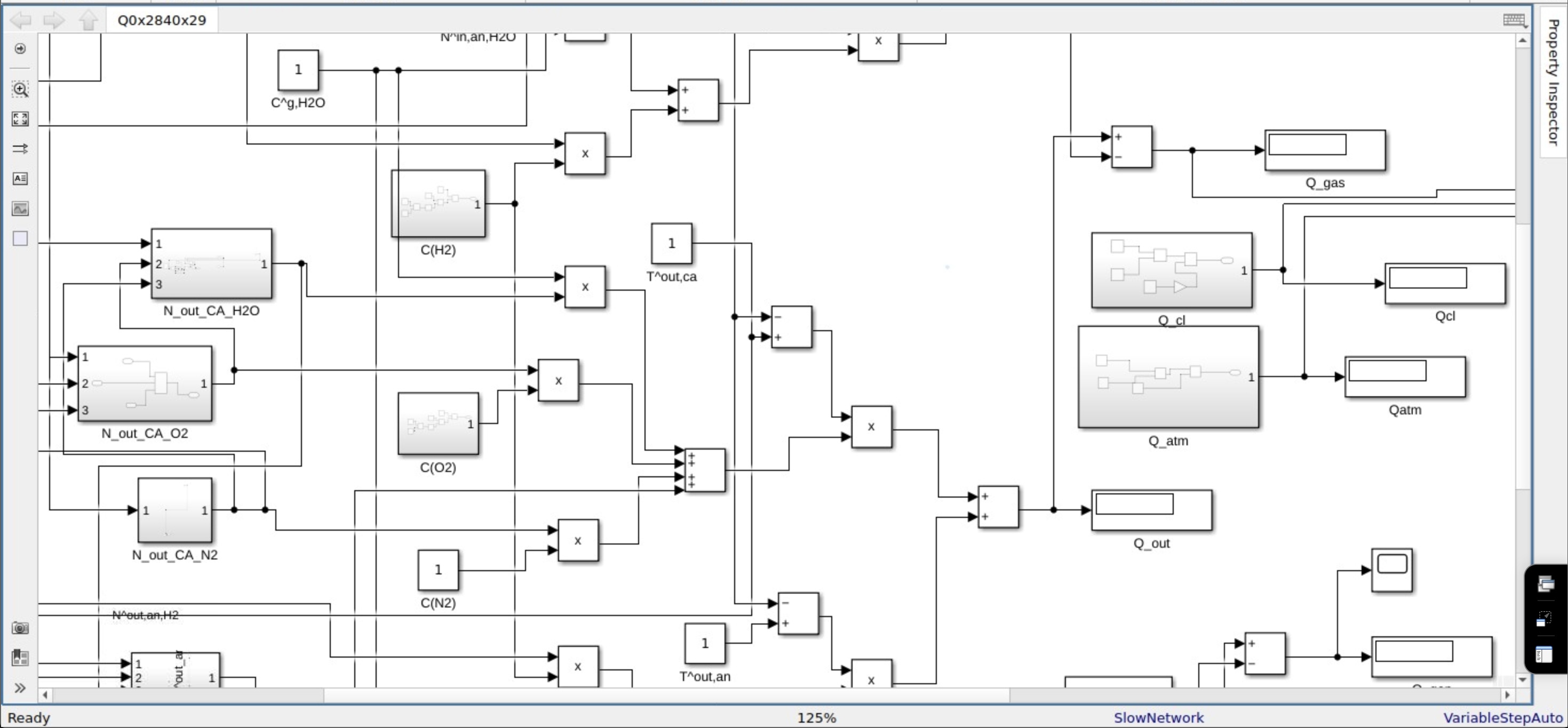
Fig. 2. Simulink model for Efficiency, this is a zoomed image of the model.
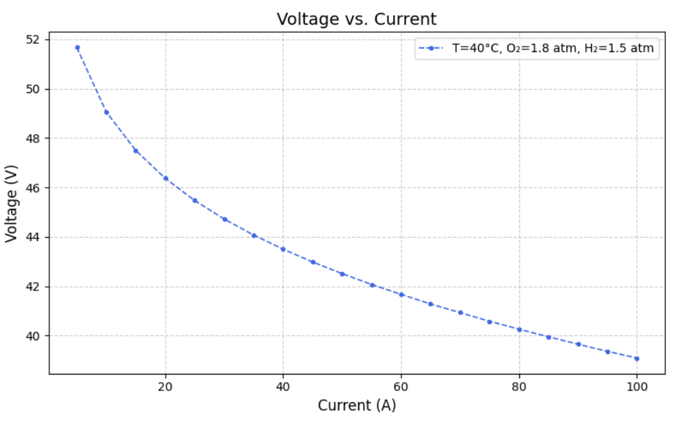
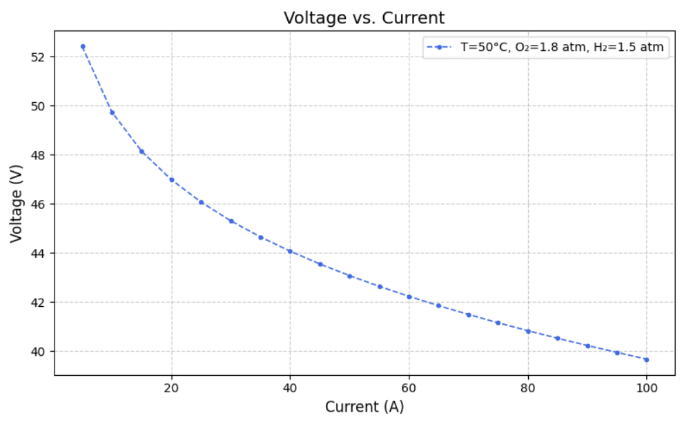
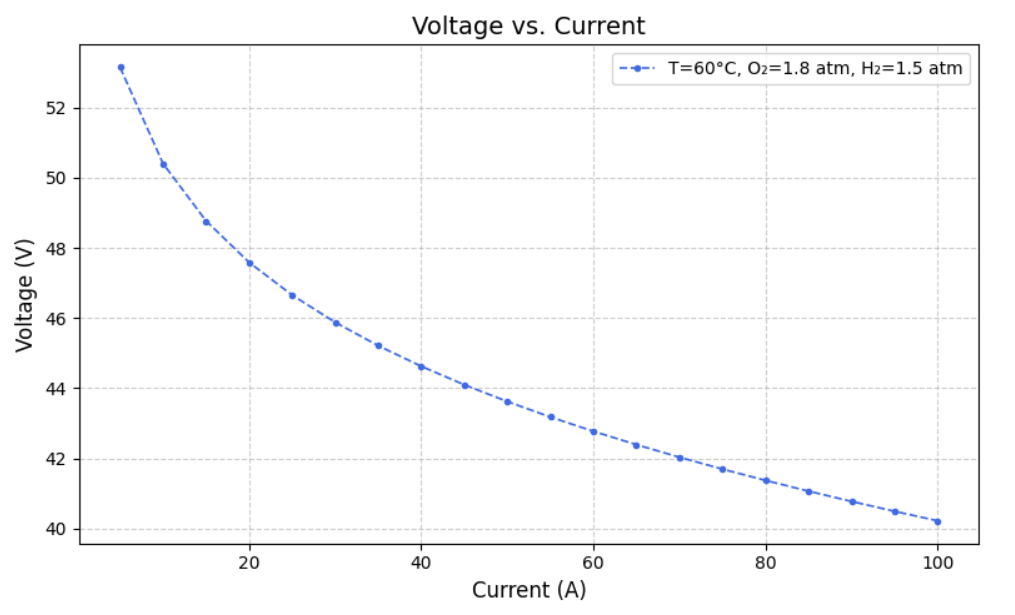
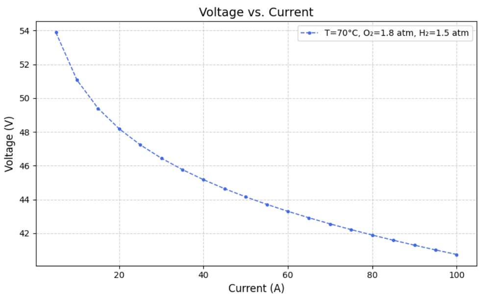
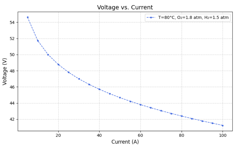
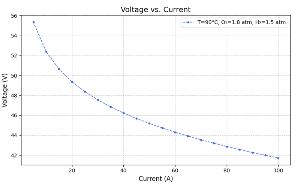
After modelling the Simulink, we created datasets for different Current, Temperature, Pressure of O2, Pressure of H2, Voltage(dependent variable) and Power(dependent variable) such that varied one and kept others constant. From this we ran the model to extract Heat Generated,Thermal Efficiency, Electrical Efficiency and Overall efficiency. Following are the graphs of Voltage(V) versus Current (A) at fixed oxygen pressure of 1.8 atm and fixed hydrogen pressure of 1.5 atm, but at different temperatures of 40, 50, 60, 70, 80 and 90 degree celcius.
IV. MACHINE LEARNING MODEL
1) Linear Regression - used to model the relationship between a dependent variable (target) and one or more independent variables (predictors). It's called "linear" because the relationship is assumed to be a straight line (linear) when plotted.
2) KNN Regression - predicting the target value for a new data point, the algorithm identifies the K nearest neighbors of that data point using a distance metric, K is a hyperparameter that needs to be set by the user. A smaller K makes the model sensitive to noise, while a larger K can smooth out predictions but might overlook local variations
3) Decision Tree Regression - predicting a continuous output variable (numerical value) by segmenting the data into smaller subsets based on decision rules. It is based on a tree structure where each node represents a decision point (split) based on a feature, and the final predictions are made at the leaf nodes.
4) Random Forest Regression - builds multiple decision trees and combines their outputs to make predictions for continuous variables. It is a robust and powerful method that addresses the limitations of individual decision trees, such as overfitting and instability.
5) Gradient Boosting Regression - builds models sequentially, with each new model correcting the errors of its predecessor. The first tree fits the data to minimize the error. The residual errors from the first tree are calculated, and the next tree is trained to predict these residuals.
6) Support Vector Regression - derived from Support Vector Machines (SVM). Unlike traditional regression methods that aim to minimize the prediction error, SVR seeks to fit a function within a specified margin of tolerance.
These six models were adopted to analyze our results.
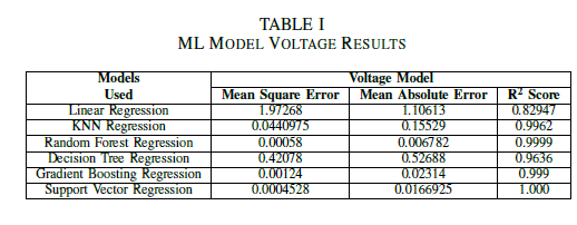
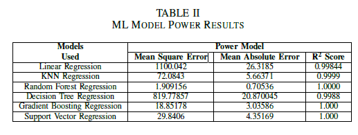
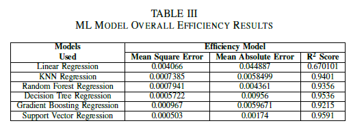
V. RESULTS
The Mean Square Error, Mean Absolute Error and R square score has been summarized in the following table for each Voltage, Power and Efficiency Model.
VI. CONCLUSION
This project successfully modeled and optimized a Ballard PEMFC system using MATLAB/Simulink, validating performance metrics like voltage, power output, and thermal/ electrical efficiency under varying conditions. Higher hydrogen and oxygen pressures (1.5–2.2 atm) and controlled cooling flow rates (0.01–0.15 L/s) boosted CHP efficiency up to 85 percent, while excessive current loading caused voltage instability. ML models like Random Forest, K nearest neighbors, and Support Vector Regression accurately predicted efficiency trends, highlighting their potential for real-time PEMFC optimization. Machine Learning models have proven to be an excellent method of simulating and predicting the behavior of fuel ,cells which are expensive to produce. We see that these models provide us with the best parameter values that can be used in our fuel cells without having to experiment with the proportions in the real world.
VII. FIGURES AND GRAPHS
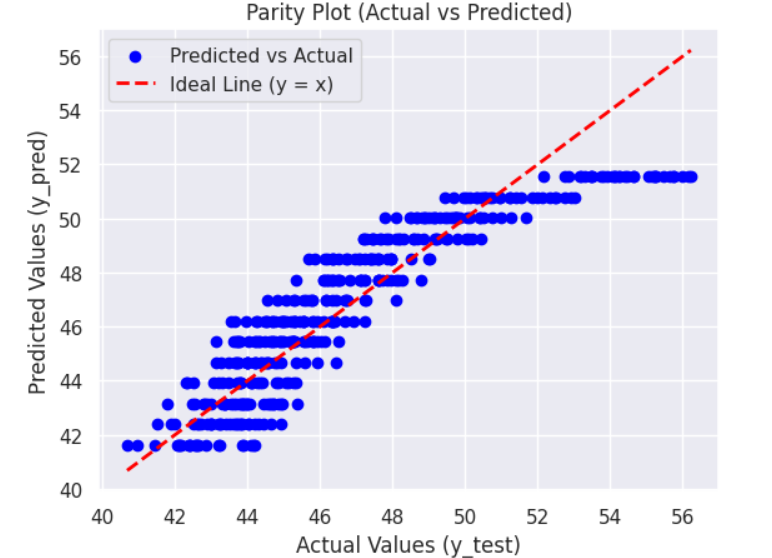
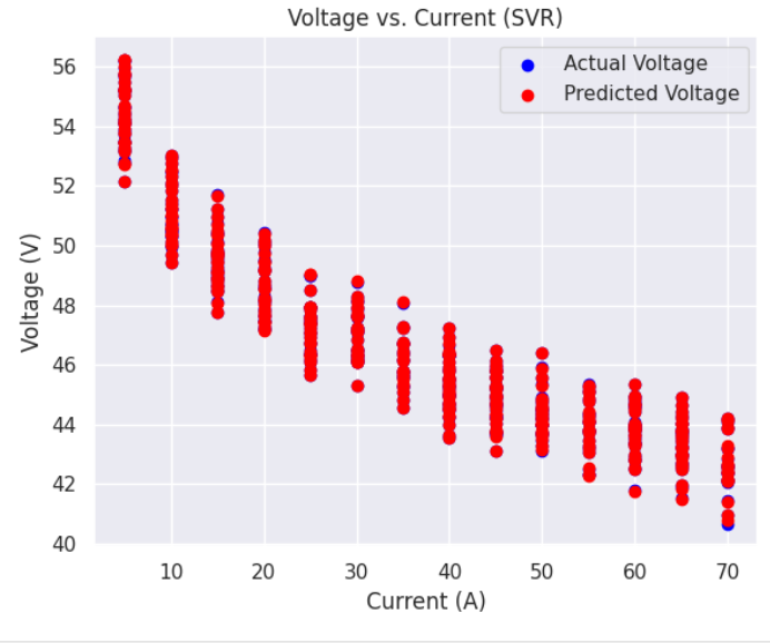
a) Voltage versus Current graphs: Following are the Voltage v.s. Current graphs for the best and least R square score.
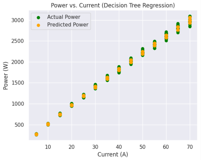
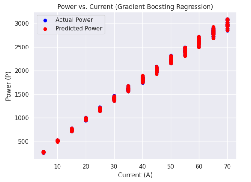
b) Power versus Current graphs: Following are the Power v.s. Current graphs for the best and least R square score.
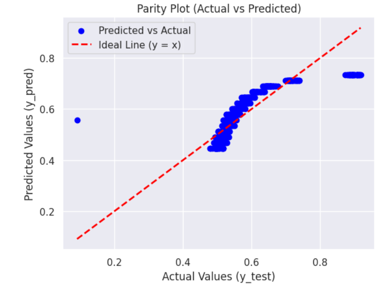
c) Overall Efficiency versus Current graphs: Following are the Efficiency v.s. Current graphs for the best and least R square score.

REFERENCES
[1] Xin Zhang , Lingyi Xu , Long Zou , Ziheng Jiang , Jiadong Liao, Pengyun Gao, Shian Li,Qiuwan Shen, “Modeling and simulation of a residential-based PEMFC-CHP system,” Volume 19, Issue 8, August 2024, International Journal of Electrochemical Science 19 (2024) 100638.
[2] Naef A.A. Qasem, “A recent overview of proton exchange membrane fuel cells: Fundamentals,”Applied Thermal Engineering 252 (2024) 123746, Volume 252, 1 September 2024 applications, and advances.
[3] Musio, F., Tacchi, F., Omati, L., Gallo Stampino, P., Dotelli, G., Limonta, S., Brivio, D., & Grassini, P. (2011). PEMFC system simulation in MATLAB-Simulink® environment. International Journal of Hydrogen Energy, 36(13), 8045–8052. https://doi.org/10.1016/j.ijhydene.2011.01.093
[4] Lv, B., Zheng, W., Sun, J., Yuan, J., Liu, Z., & Zhang, B. (2024). Modeling and Simulation of PEMFC Based on Physical Design Parameters. Proceedings - 2024 9th Asia Conference on Power and Electrical Engineering, ACPEE 2024, 1038–1044. https://doi.org/10.1109/ACPEE60788.2024.10532397
Report Information
Report Details
Created: April 6, 2025, 8:01 p.m.
Approved by: Bhavya Jain [Piston]
Approval date: None
Report Details
Created: April 6, 2025, 8:01 p.m.
Approved by: Bhavya Jain [Piston]
Approval date: None